Training
Training a model simply means learning (determining) good values for all the weights and the bias from labeled examples. In supervised learning, a machine learning algorithm builds a model by examining many examples and attempting to find a model that minimizes loss; this process is called empirical risk minimization.
Loss
Loss is a number indicating how bad the model’s prediction was on a single example. It is the difference between the predicted value and true value. If the model’s prediction is perfect, the loss is zero; otherwise, the loss is greater.
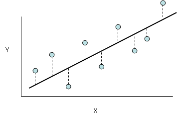
- The dashed lines represents loss
- Black line represents predictions
Accuracy
Accuracy is used to explain a model’s performance and gives the summary of predictions on the classification problems. It assists in identifying the uncertainty between classes.
Accuracy = No of correct predictions / Total predictions
Example:
If out of 100 test samples, the model is able to classify 93 of them correctly, then the model’s accuracy will be 93.0%
Note: Most of the time, accuracy increases with the decrease in loss. But, it may not be always true.
Confusion matrix
Confusion matrix is used to explain a model’s performance and gives the summary of predictions on the classification problems. It assists in identifying the uncertainty between classes.
A confusion matrix gives the count of correct and incorrect values and also the error types
Bias
The difference between the average prediction of our model and the correct value. If the bias value is high, then the prediction of the model is not accurate. Hence, the bias value should be as low as possible to make the desired predictions.
Variance
The number that gives the difference of prediction over a training set and the anticipated value of other training sets. High variance may lead to large fluctuation in the output. Therefore, the model’s output should have low variance.
Dimensionality Reduction
In the real world, we build Machine Learning models on top of features and parameters. These features can be multi-dimensional and large in number. Sometimes, the features may be irrelevant and it becomes a difficult task to visualize them.
Here, we use dimensionality reduction to cut down the irrelevant and redundant features with the help of principal variables. These principal variables are the subgroup of the parent variables that conserve the feature of the parent variables